Matt Bristow has developed a new analytical method to determine the effects of cyclic loading on both axially loaded and laterally loaded piles, including large diameter monopiles:
- Based on the use of cyclic degradation curves and a new numerical procedure to quantify the effects of cyclic loading. For laterally loaded piles this involves the determination of cyclic p-y modifiers. The methodology shows that every application has its own bespoke set of cyclic p-y curves, though most p-y curves fit within an upper and lower band range.
- Fully developed solution ready to use in the design office today. Methodology can easily be scrutinised with no reliance on black-box 3D FEA.
- 5 years ahead of the current research in the industry (reference industry news dated February 2018). Current research unlikely to match range of applicability of new method.
- Cyclic p-y modifiers determined for any pile diameter, cyclic loading, length/diameter ratio, soil type, or soil layering. Method investigated for diameters 0.3m up to 10.0m or more. Loading can be simple or complex spectrum, and unlimited number of cycles. Suitable for piles with length/diameter ratios less than L/D < 6. Cyclic degradation curves provided for many soil types, including sand, clay, materials in between soil and rock, weathered rock, and strong rock, etc. Method can uniquely be applied to layered soils, e.g. mixed soils or soils over rock, etc.
- Optimum pile length can be determined whereby the pile length is minimised and the cyclic loading is satisfactorily resisted.
Examples
In order to illustrate range of applicability of new method, a few examples are included below:
Figure 1 shows the reduction of pile response due to cyclic loading versus diameter. Not only does this show the method is suitable for any diameter, but it also shows the immediate benefit for large diameter monopiles (i.e. z/D ratio reduces with diameter).
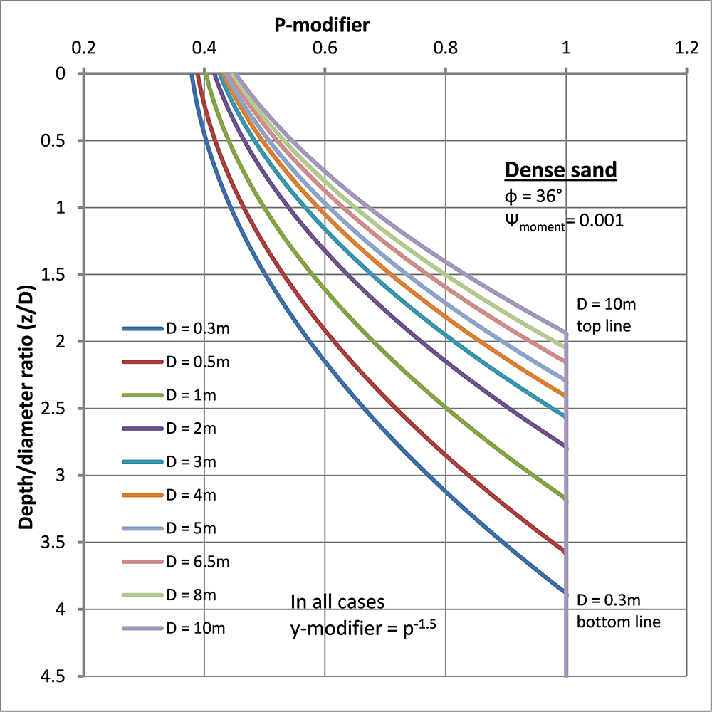
Figure 1
Figure 2 shows the influence of reducing length diameter ratio (L/D). Not only can the method be applied to any L/D ratio, but it shows how cyclic loading becomes increasingly important as the L/D ratio drops below L/D = 4.5.
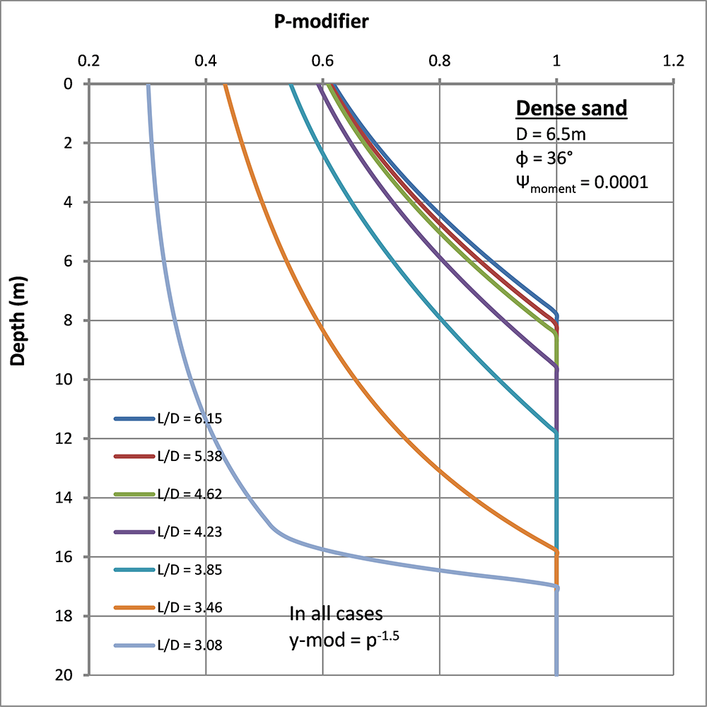
Figure 2
Figure 3 shows the reduction in p-y modifiers with increasing severity of cyclic loading (Ψmoment is a parameter used to quantify the severity of cyclic loading). As the cyclic loading becomes less severe the cyclic p-y curves tend towards the static p-y curves.
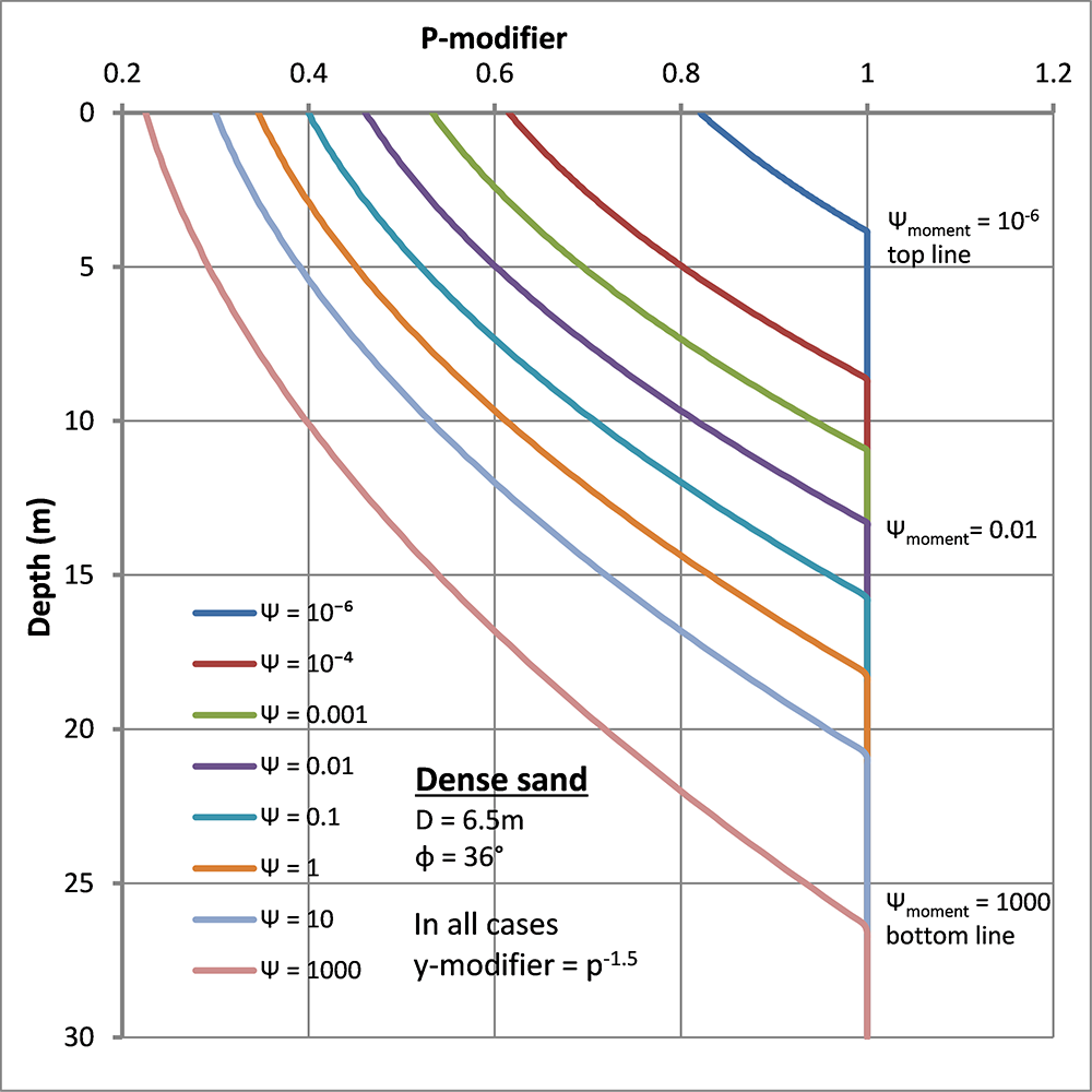
Figure 3
Figure 4 shows the different soil types the methodology has been developed for over the years (current methods barely cater for either sands or clays). Different soil types will produce different sets of cyclic p-y modifiers. Alternatively, default or lower bound cyclic degradation curves can be used for many applications.
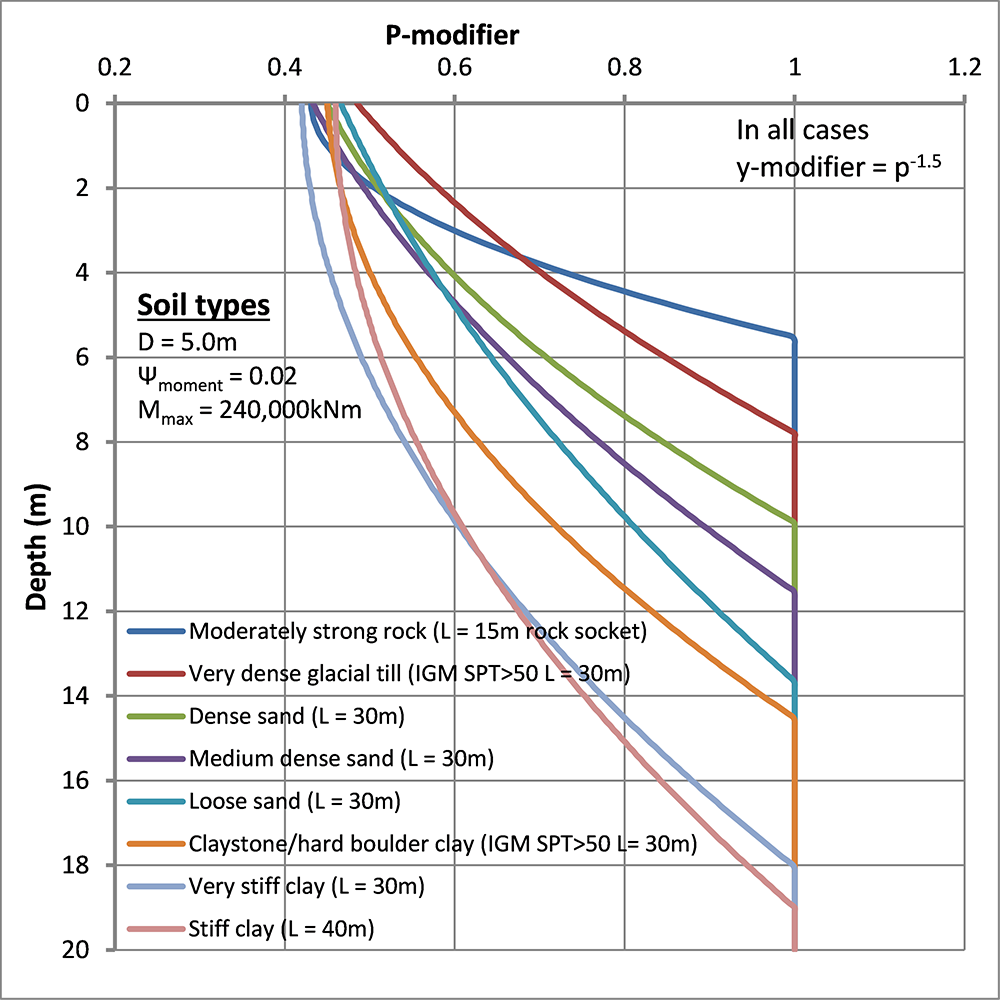
Figure 4
Figure 5 – Mixing of strong and weak soil layers can produce quite unfamiliar sets of cyclic p-y curves. Figure 5 shows the p-y modifiers for medium dense sand over weathered rock (a common occurrence across sites). Figure 5 highlights the potentially unsafe situation where the very high soil reactions at the top of short rock sockets can cause the rock to degrade at an alarming rate.

Figure 5
Advantages
The new analytical method offers a significant step forward in current knowledge. Some advantages are as follows:
- Cyclic degradation curves can be produced to suit different soil types, e.g. sand, clay, very dense glacial till, heavily over-consolidated clays, weathered and fractured rock masses, or strong rock. Only one equation is required to describe all degradation curves. Cyclic degradation curves can be based on recommended generic cyclic degradation curves for each soil type, or alternatively, determined from laboratory cyclic testing.
- The numerical method is suitable for any complexity of cyclic loading, e.g. random or variable loading, one-way or two-way loading, and any number of terms. Calculations can be performed quickly (and without need for specialist software). This is particularly suitable for highly dynamic structures such as wind turbines where the loading spectrum (e.g. Markov matrices) may contain hundreds of terms.
- The method is suitable for layered soils, e.g. soils increasing in strength with depth, mixed soils of alternating sands and clays, or weaker soils overlying stronger rock. For laterally loaded piles, layered soils can produce quite unfamiliar p-y curves compared to the standard curves, especially where there are large differences in strength/stiffness between successive soil layers.
- The optimum pile length can be found quickly and efficiently by reducing pile length until the cyclic capacity is reached. The method can be used for either short/rigid or long/flexible piles. The method shows that the effects of cyclic degradation increase rapidly as length/diameter ratio decreases below L/D = 4.5. The method has also been used for very short piers with length/diameter ratios less than L/D < 2 (with inclusion of additional force-displacement and moment-rotation curves).
- Pile response can be determined in terms of residual static capacity, i.e. the reduced static capacity after all cyclic loading has occurred. In addition, displacement due to cyclic loading and accumulated displacement can be determined. For laterally loaded piles, when cyclic loading is very low, cyclic p-y curves tend towards the static p-y curves and accumulated displacement is very small.
Articles and more
Part 1: Basic methodology
The basic methodology for laterally loaded piles is described in research paper “Cyclic Loading of Piles Using the P-Y Method”. The paper is available from DFI Journal (Volume 13 Issue 2 dated 29th May 2019) https://doi.org/10.37308/DFIJnl.20190529.204. The paper describes a new numerical procedure to quantify the effects of the cyclic loading at each soil depth and convert that to a set of cyclic p-y modifiers. The new method introduces the concept of cyclic degradation damage, which is defined as sum of the cyclic degradation that is occurring at each soil depth.
Cyclic degradation calculations are based on the shear stresses in the soil. Consequently, anything that causes the shear stresses to change (e.g. pile length, pile diameter, applied loading, etc.) will automatically be included in the calculation of cyclic p-y modifiers. The new methodology is able to reproduce by independent analysis the cyclic p-y curves presented in API RP2A (2000), but is also able to investigate what happens when it is applied to other pile configurations (e.g. pile properties, severity of loading, and soil types, etc.).
Part 2: Cyclic degradation curves
Cyclic degradation curves show the variation of the cyclic shear stress (amplitude) and mean shear stress versus the number of load cycles to failure. Matt Bristow has developed a new mathematical form for the cyclic degradation curve in which a single equation is used to plot each set of cyclic degradation curves. A typical cyclic degradation curve with mean load included is shown in Figure 6. The cyclic degradation curves can be used for both axially loaded and laterally loaded piles. A particular advantage of the new mathematical form is that it is suitable for complex loading spectrums with variable load amplitudes and unlimited number of terms. Cyclic degradation curves can be obtained from laboratory tests or pre-established curves.
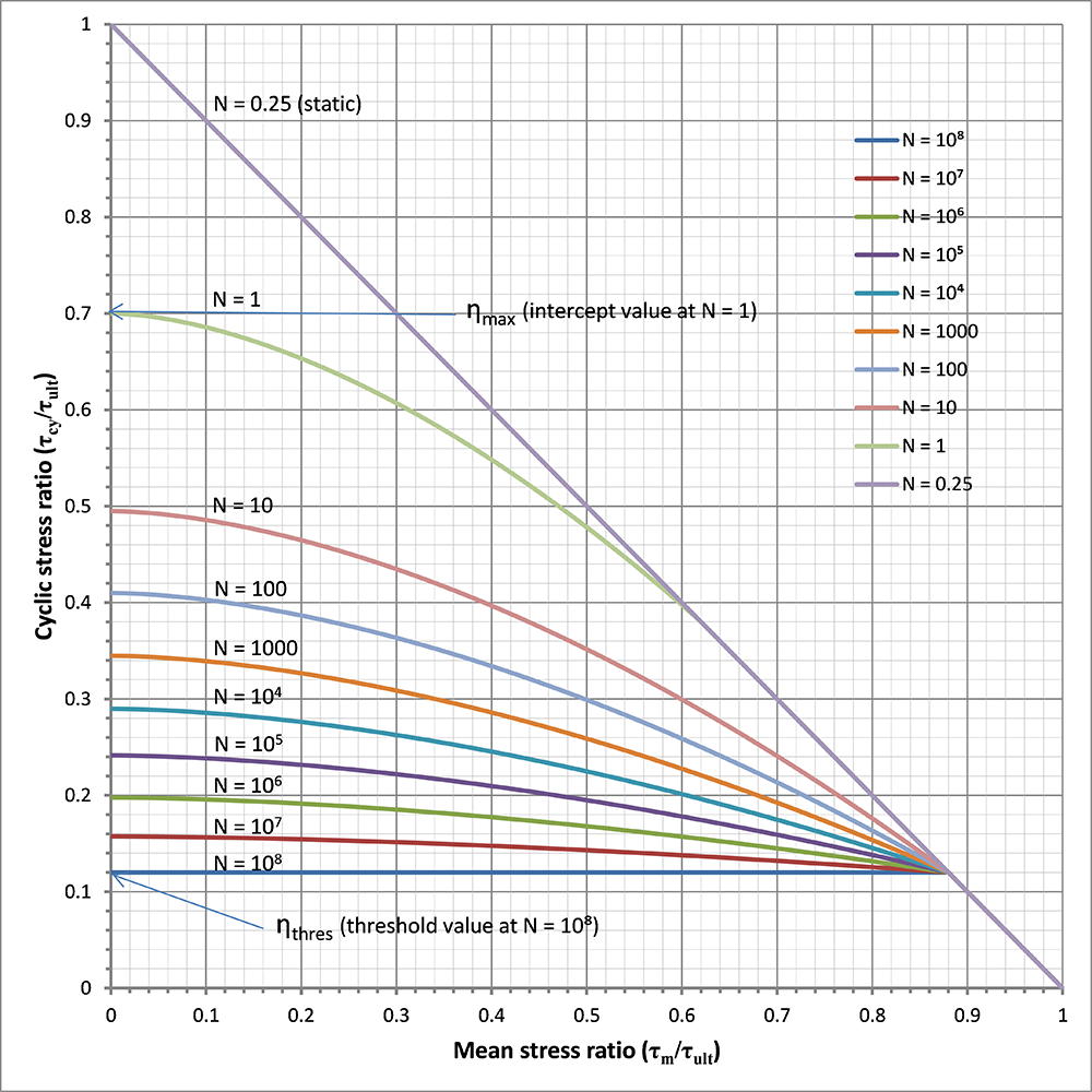
Figure 6. Typical cyclic degradation curve (including mean load)
Furthermore, sets of cyclic degradation curves (i.e. including mean load) can automatically be generated by using just one intuitive parameter. Table 1 shows the different soil types the methodology has been developed for over the years (current methods barely cater for either sands or clays). In Table 1, ηcyc is the cyclic degradation parameter used to quantify the cyclic loading resistance for each soil type. The cyclic degradation parameter of any soil normally lies in the range, ηcyc = 0.075 to ηcyc = 0.275. Figure 6 is produced using a cyclic degradation parameter, ηcyc = 0.12.
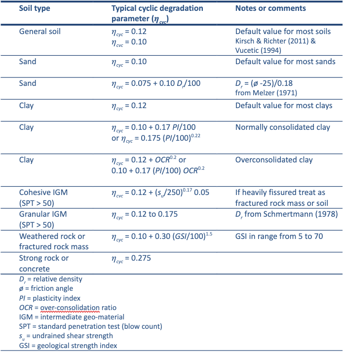
Table 1. Typical cyclic degradation parameter (ηcyc) for various soil types
Part 3: Standard cyclic p-y curves for sands and clays
Standard cyclic p-y curves have been produced for sands and clays. The standard p-y curves include factors for pile diameter, pile flexibility, and severity of loading. Standard procedures are available for both axially loaded and laterally loaded piles.
Alternatively, Matt Bristow provides consultancy services to either calculate individual cyclic p-y curves or help companies set up the new methodology in-house. Matt Bristow has developed software to considerably speed-up the calculation of the cyclic p-y modifiers.